Economic Analysis for Business Decisions Study Notes

www.marketinguyz.com

Chapter 1: Managerial Economics

Economy refers to the system of production, distribution, and consumption of goods and services within a society or a nation. It includes all the activities related to the creation and exchange of goods and services that are required to satisfy the needs and wants of individuals and businesses. The primary goal of any economy is to allocate resources efficiently to achieve maximum output with the available resources.

Economics is the social science that studies how individuals, businesses, governments, and societies allocate scarce resources to satisfy their unlimited wants and needs.

Microeconomics is the branch of economics that studies the behavior of individuals and firms in making decisions regarding the allocation of limited resources. It focuses on the analysis of the market forces that determine the price and quantity of goods and services. Microeconomics also deals with the study of how individual consumers and firms make decisions about consumption, production, and pricing.

Macroeconomics is the branch of economics that deals with the performance and behavior of the economy as a whole, rather than individual markets. It focuses on the study of the aggregate demand and supply of goods and services, and their impact on the overall economic growth and stability. Macroeconomics includes the study of variables such as inflation, unemployment, national income, economic growth, and international trade.

Managerial Economics is the application of economic principles and techniques to business decision-making. It involves the integration of economic theory with business practices to analyze and solve business problems.

Managerial Economics and Decision-making: it provides a framework for analyzing and solving business problems. Managers use managerial economics to make rational decisions that maximize the firm's profits and minimize costs.

A market refers to a place where buyers and sellers come together to exchange goods and services. It is a mechanism that facilitates the exchange of goods and services between buyers and sellers. A firm is an organization that uses resources to produce goods and services with the aim of earning a profit. The resources used by firms include labor, capital, land, and entrepreneurship.

Objectives of Firm:

Profit Maximization Model: The primary objective of a firm is to maximize its profits. The profit maximization model assumes that firms aim to produce and sell the quantity of goods and services that generates the highest profit. In other words, firms will continue to produce and sell until the marginal revenue (the additional revenue generated by selling one more unit of a good) equals the marginal cost (the additional cost incurred by producing one more unit of a good).
Economist Theory of the Firm: The economist theory of the firm suggests that firms are motivated by profit maximization, but also take into account other factors such as risk, uncertainty, and competition. This theory assumes that firms are efficient and aim to minimize costs while maximizing profits. The economist theory of the firm also suggests that firms operate in an environment of imperfect information and face transaction costs when exchanging goods and services in the market.

Chapter 2: Utility & Demand Analysis

Utility Analysis is a tool used by economists to measure the satisfaction or utility that an individual derives from consuming goods and services. Utility analysis is based on the assumption that individuals aim to maximize their overall satisfaction or utility, subject to their budget constraint (i.e., the limited income and resources available to them).

The measurement of utility is based on the principle of ordinality, which suggests that individuals can rank their preferences but cannot assign a specific numerical value to the satisfaction or utility that they derive from each good or service

Methods used to measure utility:

Cardinal Utility: This method assigns a specific numerical value to the level of utility that an individual derives from consuming goods and services. However, it is difficult to measure utility in a precise and objective manner.
Ordinal Utility: This method assumes that individuals can compare the satisfaction or utility that they derive from different goods and services and rank them in order of preference. This method is widely used in economics because it is simpler and more practical than the cardinal utility method.

The Law of Diminishing Marginal Utility is an economic concept that suggests that as an individual consumes more of a particular good or service, the additional utility or satisfaction they derive from each additional unit of the good or service decreases. In other words, as the consumption of a good or service increases, the marginal utility decreases.

Indifference Curve is a graphical representation that shows the combinations of two goods that provide the same level of satisfaction or utility to an individual. The indifference curve is based on the concept of marginal utility, and it slopes downwards from left to right, indicating that as the quantity of one good increases, the quantity of the other good must decrease to maintain the same level of satisfaction or utility.

Consumer's Equilibrium refers to the point at which an individual maximizes their utility or satisfaction, subject to their budget constraint. This occurs when the individual is consuming a combination of goods that provide the highest level of satisfaction, given their limited income and the prices of the goods.

Budget Line (AB in above graph) is a graphical representation that shows the combinations of two goods that an individual can afford, given their income and the prices of the goods.

Consumer Surplus is the difference between the total amount that an individual is willing to pay for a particular good or service and the actual price they pay for it. Consumer surplus is calculated as the difference between the maximum price that the individual is willing to pay for the good or service and the actual price that they pay.

Demand refers to the quantity of a good or service that consumers are willing and able to buy at a given price, during a specific time period. It is a crucial concept in economics as it determines the market equilibrium price and quantity. There are different types of demand in economics, including individual demand, market demand, and aggregate demand. Demand determinants include consumer income, tastes and preferences, prices of related goods, consumer expectations, demographics, and the overall economic conditions. Law of Demand means price of a good or service increases, the quantity demanded decreases, and vice versa.

Elasticity of demand refers to the degree of responsiveness of the quantity demanded of a good or service to changes in its price. The elasticity of demand can be elastic, inelastic, or unitary.

Elastic demand means that a small change in price results in a larger change in the quantity demanded, while inelastic demand means that a change in price results in a smaller change in the quantity demanded. Unitary demand occurs when the percentage change in the quantity demanded is equal to the percentage change in price.

The law of demand is a fundamental concept in economics, but there are exceptions to this law. These exceptions include the Giffen goods, Veblen goods, and the goods that have a network effect. Giffen goods are goods for which an increase in price results in an increase in quantity demanded, whereas Veblen goods are goods for which an increase in price results in an increase in demand due to their high status or prestige value. Goods that have a network effect, such as social media platforms, may have an upward-sloping demand curve as more consumers join the network.

Forecasting refers to the process of estimating or predicting future events or outcomes based on past and present data. It is an essential tool for decision-making in various fields, such as business, economics, finance, and science. Forecasting can help organizations make informed decisions about production, inventory, sales, and other aspects of their operations.

Level of Demand Forecasting:

Macro-level forecasting: This involves forecasting the overall demand for a product or service in a country or region.
Industry-level forecasting: This involves forecasting demand for a particular industry or sector, such as the automotive industry.
Company-level forecasting: This involves forecasting demand for a specific company's products or services.
Product-level forecasting: This involves forecasting demand for a particular product or service.

Criteria for Good Demand Forecasting:

Accuracy: Forecasts should be as accurate as possible to enable effective decision-making.
Reliability: Forecasts should be reliable and consistent over time.
Timeliness: Forecasts should be produced in a timely manner to enable decision-making.
Relevance: Forecasts should be relevant to the specific needs of the organization.
Understandability: Forecasts should be presented in a clear and understandable format.

Methods of Demand Forecasting:

Survey methods: This involves asking potential customers or experts about their future buying intentions or opinions on the product or service.
Statistical methods: This involves using historical data to create mathematical models to forecast future demand.
Qualitative methods: This involves using expert judgment, market research, and other non-mathematical techniques to forecast demand.

Forecasting demand for a new product can be challenging because there is no historical data available to create a statistical model. However, organizations can use a combination of survey and qualitative methods to estimate future demand. This can include conducting market research to identify customer needs and preferences, and using expert judgment to assess the potential demand for the product.

Chapter 3: Supply & Market Equilibrium

Supply refers to the quantity of goods or services that producers are willing and able to offer for sale at a given price, within a specific period. In other words, it represents the amount of goods or services that producers are willing and able to sell at different prices.

The law of supply is a fundamental principle in economics that states that there is a positive relationship between the price of a good or service and the quantity of it that producers are willing to supply, all else being equal. This means that when the price of a good or service increases, the quantity supplied by producers also increases, and vice versa.

Changes or shifts in supply refer to the alterations in the quantity of goods or services that producers are willing and able to offer for sale at different prices, due to changes in factors other than the price of the good or service itself. These factors are known as determinants of supply and include: Production costs, Technological progress, Changes in the number of producers, Changes in the prices of related goods, Changes in government policies

Elasticity of supply measures how much the quantity supplied of a good or service changes when there is a change in its price. Elasticity of Supply = (% change in quantity supplied) / (% change in price). Factors Determining Elasticity of Supply: Availability of inputs, Time horizon, Degree of specialization, Mobility of resources.

For example, a business can use the knowledge of the elasticity of supply to determine how much to adjust the quantity supplied in response to a change in price, and whether it is profitable to produce the good or service.

In a market, the equilibrium price and quantity are determined by the intersection of the supply and demand curves. When the price is too low, demand exceeds supply, and shortages occur. When the price is too high, supply exceeds demand, and surpluses occur. However, when the price is at the equilibrium level, the quantity supplied equals the quantity demanded, and the market is in balance.

Production function is a mathematical relationship that shows the maximum amount of output that can be produced from a given set of inputs, such as labor and capital, in a given time period, holding all other factors constant

The cost of production refers to the total cost incurred by a firm in the process of producing a certain quantity of output. There are two types of costs of production: explicit costs and implicit costs.

Explicit costs are the direct costs incurred by a firm, such as the cost of raw materials, wages, and rent.
Implicit costs are the opportunity costs of using resources owned by the firm, such as the cost of using the owner's time or capital.

Private costs are the costs incurred by a firm in producing a good or service, such as the cost of labor and raw materials. Social costs are the total costs incurred by society, including the private costs and any external costs imposed on society, such as pollution or congestion.

Accounting costs are the actual costs of production, including both explicit costs and implicit costs. Economic costs include not only the accounting costs but also the opportunity costs of using resources in production.

Short run costs are the costs that a firm incurs in the short term, when some factors of production are fixed, such as the size of the factory or the level of technology. Long run costs are the costs that a firm incurs in the long term, when all factors of production can be adjusted.

Economies of scale refer to the cost advantages that a firm can achieve by increasing its scale of production. This can be achieved through factors such as specialization, bulk purchasing, and improved technology.

The cost-output relationship is the relationship between the quantity of output produced and the cost of producing that output. The cost function is a mathematical expression of the cost-output relationship, which shows the minimum cost of producing each level of output.

Cost Output Relationships in the Short Run:

In the short run, some factors of production are fixed, and the cost of production can be divided into fixed costs and variable costs. As output increases, the firm incurs additional variable costs, resulting in a increasing marginal cost curve. The average variable cost curve tends to be U-shaped, while the average fixed cost curve decreases as output increases.

Cost-Output Relationships in the Long Run:

In the long run, all factors of production can be adjusted, and the firm can choose the most efficient combination of inputs. The long run cost function is typically more complex than the short run cost function, and may exhibit economies of scale or diseconomies of scale depending on the level of output. As output increases, the average cost curve may exhibit a U-shape or a downward-sloping shape.

Chapter 4: Revenue Analysis and Pricing Policies

Revenue refers to the total amount of money earned by a company from the sale of its products or services. There are two types of revenue - total revenue and marginal revenue. Total revenue is the total amount of money earned by a company from the sale of its products or services, while marginal revenue is the revenue generated by selling one additional unit of a product or service.

Price elasticity of demand refers Price elasticity of demand refers If the demand for a product is elastic, then a small change in price will lead to a significant change in demand, and vice versa. The relationship between revenue and price elasticity of demand is inverse - if the demand for a product is elastic, then increasing the price will lead to a decrease in revenue, and decreasing the price will lead to an increase in revenue. Conversely, if the demand for a product is inelastic, then increasing the price will lead to an increase in revenue, and decreasing the price will lead to a decrease in revenue.

Pricing policies refer to the strategies and guidelines used by companies to set prices for their products or services. Some of the commonly used pricing policies include:

Cost plus pricing: In this policy, the company adds a markup to the cost of producing a product or service to arrive at a selling price.
Marginal cost pricing: In this policy, the company sets the price of a product or service equal to its marginal cost, i.e., the cost of producing one additional unit of the product or service.
Cyclical pricing: In this policy, the company sets different prices for its products or services based on the time of year, demand, or other factors.
Penetration pricing: In this policy, the company sets a low price for a new product or service to gain market share.
Price leadership: In this policy, the company with the largest market share sets the price, and other companies in the market follow suit.
Price skimming: In this policy, the company sets a high price for a new product or service to maximize profits before competitors enter the market.

The primary objectives of pricing policies are:

Profit maximization: The primary goal of most businesses is to maximize their profits, and pricing policies play a critical role in achieving this objective.
Sales growth: Another objective of pricing policies is to promote sales growth. By setting prices at a lower level, businesses can attract more customers and increase their market share.
Market share maintenance: Pricing policies can also be used to maintain a company's existing market share. If a business sets its prices too high, it risks losing customers to its competitors.
Reputation management: Pricing policies can also influence a business's reputation in the marketplace. If a business consistently offers products or services at a high price, it may be seen as a luxury or premium brand. If it consistently offers products or services at a low price, it may be perceived as a budget brand. A well-managed pricing policy can help businesses establish and maintain their desired brand reputation.
Cost recovery: Pricing policies can also be used to recover costs associated with producing and delivering products or services. This is especially important in industries where production costs are high or where there is intense competition.

Primary types of markets

Perfect Competition Market: In a perfect competition market, there are a large number of buyers and sellers, and no single buyer or seller can influence the market price.
Monopoly Market: In a monopoly market, there is only one supplier of a product or service, giving them complete control over the market price.
Oligopoly Market: In an oligopoly market, a small number of large firms dominate the market. Each firm has significant market power and can influence the market price. Barriers to entry make it difficult for new firms to enter the market and compete.
Monopolistic Competition Market: In a monopolistic competition market, there are many firms selling similar but not identical products. Each firm has a small degree of market power and can influence the market price. Firms can differentiate their products through branding and advertising.

In the short run, the equilibrium in a perfectly competitive industry is determined by the intersection of the industry's supply and demand curves. Here are the key steps to understanding the short-run industry equilibrium:

Demand Curve: The demand curve for the industry represents the total quantity of the product demanded by all buyers at different prices. The demand curve slopes downward, indicating that the higher the price, the lower the quantity demanded.
Supply Curve: The supply curve for the industry represents the total quantity of the product that all firms in the industry can produce at different prices. The supply curve slopes upward, indicating that the higher the price, the higher the quantity supplied.
Equilibrium Price and Quantity: At this point, the quantity demanded and the quantity supplied are equal, and there is no excess supply or demand in the industry.
Firm's Production Decision: Each firm in the industry will decide how much to produce based on the market price. If the market price is higher than the firm's marginal cost, the firm will increase production. If the market price is lower than the firm's marginal cost, the firm will decrease production.
Short-run Profits: If the market price is higher than the average total cost of production, firms in the industry will earn short-run profits.
Entry or Exit of Firms: In the short run, some firms may enter or exit the industry based on their short-run profits or losses. If firms are earning profits, new firms may enter the market. If firms are incurring losses, some firms may exit the market.

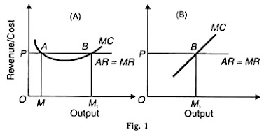
Short-run Firm Equilibrium under Perfect Competition:

The firm's equilibrium is determined at the point where its marginal cost (MC) curve intersects the market price (P) curve.
The firm will produce the quantity of output where its MC equals the market price.
If the market price is above the firm's average variable cost (AVC), the firm will produce and earn a profit.
If the market price is below the firm's AVC, the firm will shut down and incur a loss.

Long-run Industry Equilibrium under Perfect Competition:

In the long run, new firms can enter or exit the industry.
If firms are earning profits, new firms will enter the industry, increasing the supply of the product and driving down the market price.
If firms are incurring losses, some firms will exit the industry, decreasing the supply of the product and driving up the market price.
The industry will reach its long-run equilibrium when the market price equals the minimum of the average total cost (ATC) curve for each firm in the industry.
At the long-run equilibrium, each firm earns zero economic profit, as the market price equals the minimum ATC.

In the long-run under perfect competition, a firm is said to be in equilibrium when it is earning normal profits, which means that the firm is making enough revenue to cover all its costs, including the opportunity cost of the owner's resources.

The long-run equilibrium of a perfectly competitive firm is characterized by two conditions:

Marginal cost (MC) equals average total cost (ATC): In the long run, firms in a perfectly competitive market are able to adjust their plant size to produce at the minimum efficient scale, which means that the average total cost of production is minimized. Therefore, in long-run equilibrium, the marginal cost of production is equal to the average total cost.
Price (P) equals marginal cost (MC): In the long run, firms in a perfectly competitive market are price takers, which means that they have no control over the market price of the product. Therefore, in long-run equilibrium, the price of the product is equal to the marginal cost of production.

When these two conditions are met, the firm is earning normal profits, which means that its revenue is equal to its total costs, including the opportunity cost of the owner's resources.

Price Discrimination under Monopoly:

Price discrimination occurs when a monopolist charges different prices to different groups of consumers for the same product. The monopolist can do this because they have market power and can segment the market based on different consumer groups' willingness to pay. Price discrimination can increase the monopolist's profits but may also lead to consumer surplus loss. Example, Coke at general store and movie theater

Bilateral monopoly occurs when there is only one buyer and one seller in the market. The buyer and seller must negotiate a price, and both have some degree of market power. The price that is ultimately agreed upon is determined by the relative bargaining power of the two parties.

Pricing power is the ability of a firm to influence the price of its product. Firms with pricing power have some degree of market power, which allows them to charge a higher price than their marginal cost of production.

Duopoly is a market structure in which there are only two firms selling a particular product. Duopolies can lead to price wars and other anti-competitive behavior, and governments may need to intervene to prevent such behavior.

Need for Government Intervention in Markets:

Governments may need to intervene in markets to prevent anti-competitive behavior, promote competition, or protect consumers from price gouging. Government intervention can take the form of antitrust laws, price controls, and other regulatory measures. Governments can prevent or control monopolies by enforcing antitrust laws, breaking up large firms, promoting competition, and regulating prices. Governments can also encourage the entry of new firms into the market to increase competition and reduce the power of existing monopolies.

Chapter 5: Consumption Function and Investment Function

The consumption function is a relationship between disposable income and consumer spending. It shows how much consumers spend on goods and services at different levels of disposable income. The consumption function is an essential tool for understanding how changes in income and wealth affect aggregate demand.

The investment function is a relationship between the interest rate and the level of investment spending. The investment function shows how much firms are willing to invest in capital goods at different interest rates. Changes in the interest rate can have a significant impact on the level of investment and, consequently, on the overall level of output and employment.

The marginal efficiency of capital (MEC) is the expected rate of return on an additional unit of capital. The MEC is an essential concept in investment analysis because it determines whether firms will invest in new capital goods. Business expectations refer to the expectations that firms have about future economic conditions, such as interest rates, tax policies, and government regulations. Business expectations can affect investment decisions and overall economic activity.

The multiplier is a concept that measures the impact of an initial change in spending on the overall level of output and employment. The multiplier effect occurs because a change in spending leads to a change in income, which in turn leads to additional rounds of spending. The multiplier can be calculated using the formula 1/(1-MPC), where MPC is the marginal propensity to consume.

The accelerator is a concept that measures the impact of changes in the level of investment on the overall level of output and employment. The accelerator effect occurs because an increase in investment leads to an increase in the demand for capital goods, which in turn leads to an increase in the demand for labor and other inputs. The accelerator can be calculated using the formula change in investment/ change in output.

A business cycle refers to the recurring pattern of expansion and contraction in economic activity over time. It is a natural phenomenon that occurs due to various internal and external factors affecting the economy. It is composed of four phases: expansion, peak, contraction, and trough.

Phases of Business Cycles:

Expansion: During this phase, economic activity is increasing, output, employment, and incomes are rising, and consumer and business confidence is high. This phase is characterized by increasing investment, rising prices, and low unemployment rates.
Peak: The peak marks the end of the expansion phase and the beginning of the contraction phase. During this phase, economic activity slows down, and output, employment, and incomes begin to level off or decline. Consumer and business confidence may start to decline, and investment may decrease.
Contraction: The contraction phase is characterized by declining economic activity, falling output, employment, and incomes, and rising unemployment rates. This phase is marked by decreasing investment, declining prices, and low consumer and business confidence.
Trough: The trough marks the end of the contraction phase and the beginning of the expansion phase. During this phase, economic activity begins to pick up, output, employment, and incomes start to rise, and consumer and business confidence may improve.

Measures to Control Business Cycles:

Governments and central banks can use various measures to control business cycles, such as fiscal and monetary policies. Fiscal policies include government spending and taxation policies, while monetary policies include interest rate policies and open market operations. These policies can be used to stimulate economic activity during periods of contraction and to dampen economic activity during periods of expansion.

Business cycles have significant implications for business decisions, as they affect the overall level of demand, output, and employment. During periods of expansion, businesses may invest in new capital goods, expand production, and hire new workers. During periods of contraction, businesses may cut back on investment, reduce production, and lay off workers. Therefore, businesses need to be aware of the current phase of the business cycle and adjust their strategies accordingly.